Input data

Preparing the spreadsheet.

Reading study information into R.

Once the files have been processed, the easiest way to proceed is by settting up a text file containing all the necessary information about each scan. This file should be comma or space separated, have one row per scan, with each column containing info about each scan. One of the columns should contain the filename pointing to the MINC volumes to be processed. An example might look like the following:

file,Genotype,scale
filename1.mnc,+,0.98
filename2.mnc,-,0.91
filename3.mnc,-,0.92

Notice how the first row contains a header. This is optional, but makes later access to the data easier and is therefore recommended.

The next step is to actually load this filename into R. The steps are given below:

The two library commands load the RMINC and xtable libraries into R. xtable is only necessary for display purposes in this manual (which, by the way, is being written using Sweave, a tool for combining R with latex). The variable glim.file is then assigned the location of the input data file, which in turn is read into the gf variable.

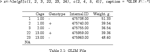
The little code fragment and table above just shows what a subset of the gf variable looks like. To get a feel for the data and some of the RMINC functions, the first file is then read and a histogram produced (for the curious, the files used in this example actually consist of log Jacobians of deformation fields, not voxel density maps usually used in VBM).