The two-compartment model used is expressed by the following equation:

where K1 is the rate constant of flow from vasculature to tissue, k2 is the rate constant of flow from tissue to vasculature, A(t) is the activity in the brain, and Ca(t) is the activity in the blood.
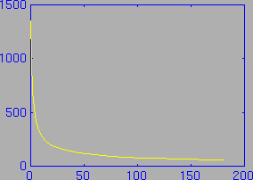
We wish to solve this equation for K1 and k2, given the A(t) and Ca(t) curves. Usually the blood activity (Ca) and brain activity (A) curves are expressed by measuring their values at about ten points in time. An example blood activity curve is shown in the following figure:

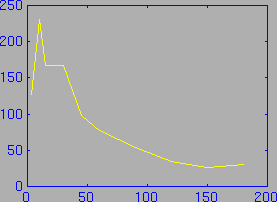
And an example brain activity curve:

This data can be easily entered into MATLAB, since MATLAB has the ability to read in text files that contain columns of numbers. For example, the brain curve above is represented by the two columns of numbers:
3       127
10      231
15      167
30      167
45      98
60      77
90      54
120     35
150     26
180     31
where the first column is the time of the sample in minutes, and the second column is the activity of the sample. If this data was saved in a file called ratbrainact.txt, then it could be loaded into MATLAB with the command:
load ratbrainact.txtThis loads the data, and creates a 10x2 matrix called ratbrainact (for more details on reading data files, please see the MATLAB User's Manual). The previous plot could then be created with the command:
plot (ratbrainact(:,1), ratbrainact(:,2))which plots the second column versus the first one.
In order to perform a two-compartment analysis, however, we require both the brain data and the blood data. The blood data can be loaded in exactly the same way as the brain data was. Assuming that we have the blood activity data stored in a file called ratbloodact.txt:
load ratbloodact.txtwill load the data.
Now that the data is loaded, analysis is easy. The ratbrain function will perform the analysis on the data, and return many useful variables:
[K1, k2, conf, ts_even, new_brain, theta, Vd, new_Vd] = ratbrain ...
(ratbloodact(:,1), ratbloodact(:,2), ratbrainact(:,1), ratbrainact(:,2));
The values of these variables can be retrieved very simply:
>> K1

K1 =

    0.0477

>> k2

k2 =

    0.0765

>> conf

conf =

    0.0470    0.0484
    0.0753    0.0778
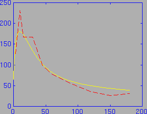
The ratbrain function also returns several other variable of interest. For example, it returns a new brain activity curve based on the calculated values of K1 and k2. This can be plotted superimposed on the measured brain activity curve to get a visual check on the quality of the curve fit. In the following figure, the measured brain activity curve is shown in red (dashed), and the calculated brain activity curve is shown in yellow.

This figure was produced by the following sequence of MATLAB commands (after running the above ratbrain command):
plot (ts_even,new_brain);
hold on;
plot (ratbrainact(:,1), ratbrainact(:,2),'r--');
Note that the calculated brain activity curve is expressed in the evenly sampled time scale ts_even.
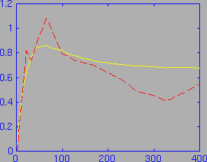
Since Vd and theta are also returned by the ratbrain function, these curves may also be plotted. As with the brain activity curve, a Vd curve based on the calculated brain activity is also returned. Therefore, a Vd versus theta curve may be plotted showing both the measured Vd versus theta, and the Vd versus theta based on the calculated values of K1 and k2. In the following figure, the measured Vd versus theta curve is shown in red (dashed), and the calculated Vd versus theta curve is shown in yellow:

This figure was produced by the following sequence of MATLAB commands (after running the above ratbrain command):
plot (theta,new_Vd);
hold on;
plot (theta,Vd,'r--');