Canny operator: definition and experiments on Matlab
- Canny operator is an edge detection tehcnique containing three processes: edge detection, thresholding, and edge thinning.
The desired localization is defined as "the points marked as edge points by the operator should be as close as possible to the center
of the ture edge." To detect and localize the edge, an edge detector is first applied. Becasue there some amount of noise exisit in
any image, it is very improtant to reduce the noise as much as possible. To do this, the edge detection process has the ability to
somewhat smooth the image and reduce the noise. Since noise, usually contains a large range of frequency and mostly high frequencies,
this makes it difficult for the detector to result a good edge detected image. This is becacuse of sometimes difference within the
magnitude of pixels constructing an edge contour and the result of edge detection may be an edge missing some pixel which is called
streaking. Also, the amount of noise can be different within image; however, the gaussian filter in the canny operator reduce some
amount of noise but not completely. The next step, thresholding is closely related to noise in the image. Even with noise estimation,
the edge detector will be susceptible to streaking if a single threshold is used. Streaking is a common problem that Canny operator
should deal with and it is done using thresholding. Indeed, streaking is the breaking up of an edge contour caused by the operator
output fluctuating above and below the threshold along the lenght of the contour. A possible way is to apply thresholding with hysteresis.
If any part of a contour is above a high threshold, those points are immediately ouput, as is the entire connected segment of contour
which contains the points and which lies above a low threshold. In this case, the probability of streaking is highly reduced since for
a contour to be broken it must flictuate above the high threshold and below the low threshold. Also, the probability of isolated false
edge points is reduced because the strength of such points must be above a higher threshold. Usually, the thresholds are set according
to the amount of noise in the image, or as a fraction of gradient magnitude of the image pixels.
- In edge detection process, first, a Gaussian kernel is used in order for noise smoothing (reduction), and the edge strength
is computed using differentiation of image in two orthogonal(vertical and horizontal axes). Then, computing the gradient magnitude as
the root sum of sqaures of the derivations is performed. The gradient direction is also calculated using the arctangent of the ratio
of the derivatives.
- The purpose of using hysteresis, in thresholding process, is to ensure that noisy edges are not broken up into multiple edge fragments.
Theoritically, the high threshold can be set quite high and the low threshold quite low for good results. But setting low threshold too
high causes edges to break up, and setting high threshold too low inceases the number of spurious (false) and undesired edge fragments
apprearing in the output image.
- In edge thining process, also called "non-maximum supression," is performed on the pixel with the gradient magnitude, in
order to thin the edge. Non-maximum suppression based on the gradient magnitude explores for all pixels in the direction of steepest
gradient. A pixel is marked as possible edge point (set to 1), if it has a larger gradient than both: its neightbours located in the direction closest
to that of the gradient, and its neightbours located in the opposite direction. Otherwise, the pixels are set to zero and the final result will
be a binary image.
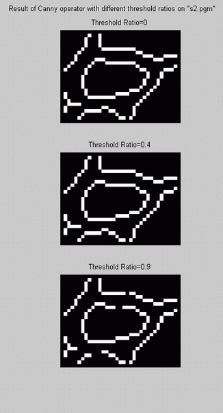
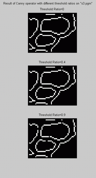
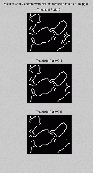
- In Matlab, there is a default code called "edge" which is used for Sobel, Roberts, Prewitt, LOG, Canny and so on. The default
threshold ratio in Matlab "edge" code, for canny operator, is 0.4. A modified version of "edge" was created to jsut apply the canny operator on
the desired image. This code is called "canny.m" with the flexibility in assigning the threshold ratio (the difference between high and
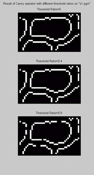
low threshold). Afterwards, "canny" code with three different values for threshold ratios: 0, 0.4 and 0.9 was applied on s1.pgm,
s2.pgm, s3.pgm and s4.pgm. As mentioned above, by decreasing
the hysteresis width (the difference between the two threshold levels) edges tend to break up. Also Matlab default ratio (0.4) seems
reasonable compared with the result of threshold ratio=0, the state that the low threshold is equal to zero and the hysteresis
is maximum.


- Due to the fact that Snake programme should operate on gray scale image as well as in the binary image; there is no need for an
extra process to make a bianry image, in order to apply snake. Also there may be some information deleted in this binary image.
- Using the above concept, first, the thresholding process was suggested to be excluded in "Canny" code in Matlab, and just the edge
detection and edge thinning processes should be kept. Since the edge thining process is designed using the logical functions (e.g., AND,
OR); therefore, there is no way to exclude the binary image.
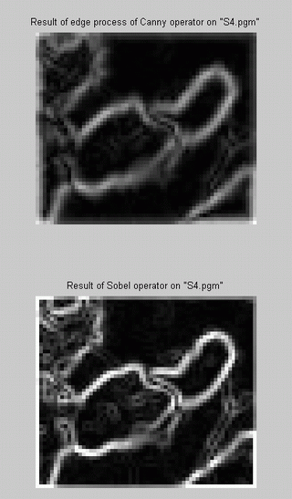
- Moreover, only the edge detection process of Canny operator, i.e., edge detection, was applied on s4.pgm to
compare the result of this process with that of Sobel operator. Results are almost a similar. However, the pixel magnitude seems to be greater
in result of Sobel, but more even in the result of Canny edge detection process.

- Canny operator algorithm can be built using different approaches. For instance, in Matlab programme, the defulat code "edge.m"
containing Canny operator, first, the images convolves with the 1st derivative of a gaussian function (filter), with the Std=1.0, as default.
then, the thresholding (high and low) values are calculated with the fixed threshold ratio=0.4 (high threshold / low threshold), and later,
the non-maxium supression, edge thinning, process is applied, mixed with the thresholding, to the filtered images.
- In the other programme (written by Ma Yi and John Koo) first, 1st derivative of a 2D gaussain function with Std=1.0, for both X
and Y directions ( as filters) are convuled individually with the image, and moreover, the results of filtering are combined using the same
combination concept as in gradient. The thresholding process is described as follows:
- finds the maximum and minimum values within the gradient matrix (edge detected image);
- setting a value called "level" that is computed as: the difference between maximum and minimum values is multiplied by a default factor (alfa=0.1),
then the result is aded to the minimum value;
- creates a matrix the same size of the image with all the elements equal to "level", comapre it with the gradient matrix and selects
the largest elements (pixels) either from gradient image or the calculated level matrix and place them in a new matrix; therefore, in this new
matrix, "after thresholding" matrix, the minimum value will be equal to level. It is, indeed, shifting up all the elements less than a
certain value ("level") to this certain value.
- Furthermore, non-maximum supression (edge thinning) is applied and the final result will be a binary image. The procedure is
as follows:
- It creates three matrices as: X=[-1 0 1; -1 0 1; -1 0 1], Y=[-1 -1 -1; 0 0 0; 1 1 1] and Z which is 3 by 3 rectangular matrix for any neighbpring
elemets of thresholded matrix greatger than "level". These matrices are to create the axes for interpolation;
- Then, it calculates XI and YI (both 2X1)repectively as the horizontally and vertically filtered image (from the edge detection
process) normilized by the Gradient value, for every element of the edge detected image. the later matrices contain the calculated value
in positive and negative form;
- the programme interpolates at the above mentioed matrices and result ZI matrix with to elements; if, for any given element of thresholded
matrix, it is larger than two elements of ZI, then it is selected and replaced by the max value of gradient matrix, otherwise, the min value of replaces it.
- In modification I made on this code, now entitled "cannymt.m" in the later part, instead of replacing the selected element by the Max of gradient matrix, the
actual value of the thresholded matrix is kept, but for the rest is the programme serves the same.
- It is suggested that the results of Snake (with or without considering the parameters: pressue, GVF) and Canny operator be compared
for individuals arbitrary regions within 110.pgm.
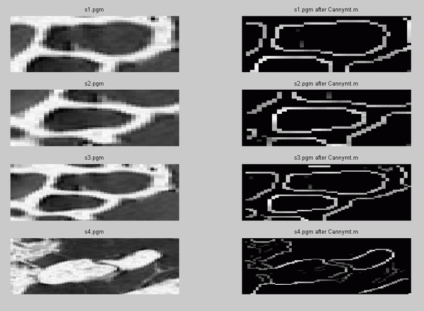
- The modified "cannymt.m" code was applied to s1.pgm through s4.pgm and the results
are the unbinary thresholded thinned images:

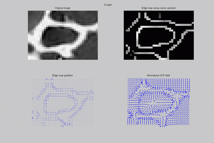
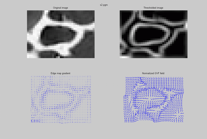
- The Gradient and GVF edge maps of s2.pgm were calculated prior to snake implementation. Results are shown below,
a slight difference exists between the edge map gradient (with arrows) of thresholded image with that of Canny image. Also, for GVF field,
external forces are better defined and located for the Canny image than the thresholded image, so that it affect
the snake result.


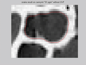
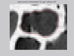
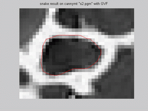
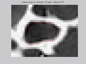
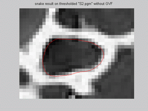
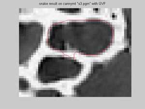
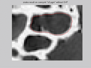
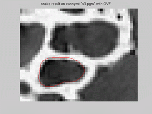
- Snake model, in matlab code, was applied for images s1.pgm through s4.pgm in different procedures:
for cannymt output image (canny edge detected) with and without GVF, and for thresholded image with and without GVF. For almost all the regions
snake for thresholded image with GVF failed, since the external forces cannot defined a proper boundary around the region. This is because of
the poor image element for some part of the boundary that are not well detected by GVF process.
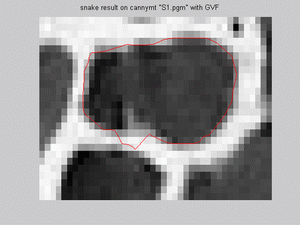
- For s1.pgm snake model on Canny image with GVF fits well except for a part the lower boundary region. For
thresholded image with and without GVF has almost similar promising results:


- For s2.pgm snake model on Canny image with and without GVF and on thresholded image has almost the same promising
results, but the difference mostly is the shifting about one pixel up or down, though it is reasonable for segmentation:


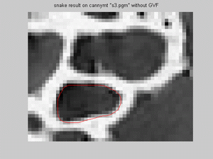
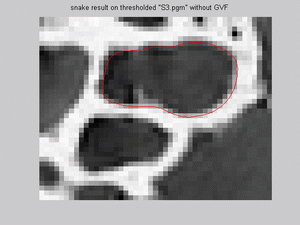
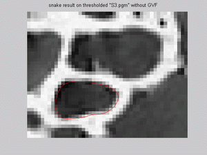
- For s3.pgm snake model was implemented for both smaller and bigger dark regions, on Canny image with/without
GVF and on thresholded image. Results show that snake model fits reseanobaly for all situations; however, the same mifit exist for canny
with GVF, as was in s1.pgm for the same situation:


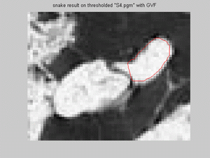
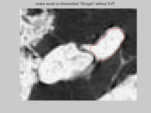
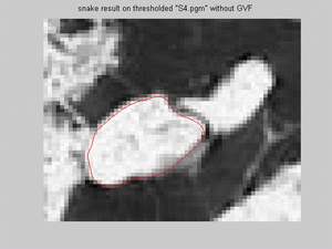
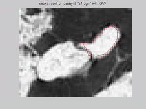
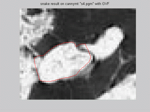
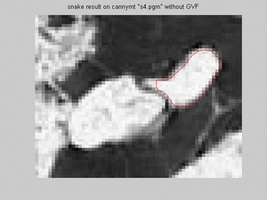
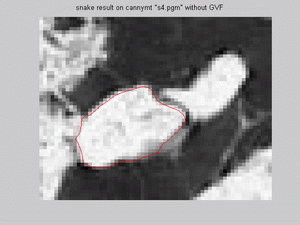
- For s4.pgm snake model was implement for both: the bigger and the smaller bright regions, on Canny image with/without
GVF and on thresholded image. Snake model does not fit the edges in the implementation for canny edge detected image:


but for snake model on canny image without GVF has promising results for both reason, but the same fitting problem as in previous report
with the sharp coner of the upper, smaller region. For the left boundary of the bigger region snake fits quite well, though usually failed
for some other implementations for other edge processing methods:


furthermore, for thresholded image with GVF, snake model didn't fail for smaller, upper regions, thoguh snake does not fit well; and for the
thresholded image without GVF, the result are similar to those with canny operator without GVF:
