Results

To obtain a quantitative evaluation of the performance of the segmentation method a training set of 40 normal subjects was selected from the ICBM database and validated with a target set of 10 different normal subjects.

VOIs were defined on T1-weighted MR images with isotropic resolution of 1 mm³. Those volumes were linearly registered into stereotaxic space to reduce positional variations which would propagate as unwanted noise in the morphometric PCA modelling. Initial testing was centered on the left hippocampus (VOI of 55 x 79 x 68 voxels). The extent of this volume captured the hippocampus and neighboring structures irrespective of normal inter- and intra-individual variability.

The method described above was used to build a model of hippocampus appearance. Table 1 lists the number t of eigenvectors required by each stage of the model to explain the chosen percentage f (eq. 8) of the observed variations. The factor r (eq. 6) was estimated as 0.006. It is important to note that the large number of eigenvectors is a direct consequence of their expressing the variations in the difference from the mean element, and not the elements themselves.

Table I: Number t of eigenvectors per model

Model	f %	# t
Grey-level	97.5	38
Warp - X	97.5	24
Warp - Y	97.5	21
Warp - Z	97.5	24
Concatenated	99.9	36

The range of values of ${\bf\delta C}$ to be used during training was set experimentally to $\pm 2$ standard deviations of the super-parameters ${\bf C}$.

As mentioned above, the appearance-based (AB) model and the ANIMAL software from Collins [3] were used to segment the hippocampus from 10 subjects for validation and comparison purposes. Manual labels for those subjects were available [5]. Kappa statistic estimates of the overlap between ANIMAL or AB segmented structures and manual labels are presented in Table III. Mean segmentation time, excluding off-line training in the case of AB, is also presented. Experiments were run on a Pentium III 550 MHz PC using MATLAB (AB) and compiled C code (ANIMAL).

Table II: Comparison of segmentation methods

n = 10	Manual	ANIMAL	AB
$\bar \kappa$	-	0.69	0.65
$\sigma_\kappa$	-	0.03	0.05
$\bar t$ (min)	120	120	19.5

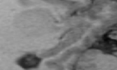
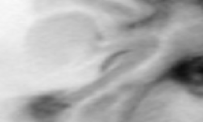
Figure 1 is a grey-level sagittal image of the region near the hippocampus medial axis of Subject 341, stereotaxically registered. Figure 2 shows the image generated by the AB model. Figure 3 shows the difference between Figs 1 and 2.

Figure 1: Subject 341 - Original grey-level image (Top = superior, Left = Anterior).

Figure 2: Subject 341 - Synthesized grey-level image (Same orientation as Fig. 1).

Figure 3: Subject 341 - Difference image (Original - Synthesized) (Same orientation as Fig. 1, intensity scale 10¹ greater to enhance small differences).

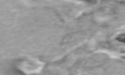Figure 4 shows the left hippocampus from Subject 341, segmented using ANIMAL non-linear registration in light grey, superimposed on the manually segmented left hippocampus in dark grey. Structure overlap is displayed in black. Figure 5 displays segmentation using the AB technique (same coloring). Values of $\kappa$ for this subject are close to the mean for each technique.

Figure 4: Subject 341 - ANIMAL (light grey) vs manual (dark grey) segmented hippocampus, overlap in black ($\kappa = 0.68$).
Figure 5: Subject 341 - Appearance-based (light grey) vs manual (dark grey) segmented hippocampus, overlap in black ($\kappa = 0.65$).