We can consider an ideal imaging process as a measurement of a continuous function describing some physical property of the brain. For instance, this property is the x-ray linear attenuation coefficient for CT and x-ray imaging, and the T1 or T2 weighted proton density for standard MR imaging. Even though the images may be actually acquired slice by slice, the ensemble of slices generally constitutes a three-dimensional data set. Each voxel of the acquisition has an intensity value (that is related to the physical property measured) and is associated with a coordinate in scanner space.
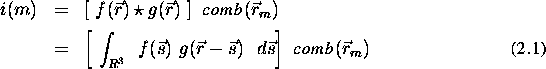
The data set can be mathematically modeled as follows. Let  be the scalar function of space describing the property to be
measured. Since any real imaging system has a limit in the spatial
frequencies that can be measured,
be the scalar function of space describing the property to be
measured. Since any real imaging system has a limit in the spatial
frequencies that can be measured,  must be convolved with
the point source response function
must be convolved with
the point source response function  of the imaging system
to obtain the measured distribution [65]
of the imaging system
to obtain the measured distribution [65]![]() . In CT imaging, the
frequency limitation comes from the finite size of the detectors and
the size of the focal spot. In MRI, it is a consequence of the limited
k-space region that is scanned. The fact that the image is made of
voxels is equivalent to multiplying by an array of delta functions.
Putting this together, the intensity associated with each voxel, in
the ideal case, is
. In CT imaging, the
frequency limitation comes from the finite size of the detectors and
the size of the focal spot. In MRI, it is a consequence of the limited
k-space region that is scanned. The fact that the image is made of
voxels is equivalent to multiplying by an array of delta functions.
Putting this together, the intensity associated with each voxel, in
the ideal case, is
where m is a label identifying each voxel and  represents the function formed by a three-dimensional array
of
represents the function formed by a three-dimensional array
of  -functions located at the center
  of each voxel.
im_model reflects the fact that the measured object property
is only known at a finite number of space locations. It must be
emphasized that the spacing between the delta-functions in the
comb must be small enough so that the Nyquist condition is
satisfied
of each voxel.
im_model reflects the fact that the measured object property
is only known at a finite number of space locations. It must be
emphasized that the spacing between the delta-functions in the
comb must be small enough so that the Nyquist condition is
satisfied![]() .
.