Selection of N3 distance for 3-Tesla scans

The selection of the N3 distance for 3-Tesla scans is often problematic as its value depends on the scanner type, the head-coil receiver, the scanning protocol, etc. While values of 50 have been suggested in the past, it appears that values between 100 to 125 are now more appropriate with current technology (current=2012). The determination of this parameter would usually be made on the basis of visual inspection after running a subject at different values and choosing the value that looks to best correct the non-uniformities. This approach was very subjective, although suitable values could be determined as such by an experienced user.

A new approach is hereby suggested to determine the optimal value of the N3 distance in a more quantitative way. A small number of subjects with good scans (say 20, no motion artifacts, for example) are selected and run with CIVET at various N3 distances like 50, 75, 100, 125, 150, 175, 200. The ensuing cortical thickness maps are analysed with the hypothesis that numerical variability (due to processing) will be minimized near the optimal value of the N3 distance, with the anatomical variability of the 20 subjects remaining inherently the same. The optimal N3 distance is chosen as the one that minimizes the average variance of the cortical thickness at all vertices of the cortical surfaces of the 20 subjects.

Required installations

• MATLAB: http://www.mathworks.com/products/matlab/
• Surfstat:

Required files

• Download CIVET average surfaces on which to display your group data: CIVET12_av.obj

Directory structure

Create a directory in your home directory called “surfstat,” and within “surfstat” a subdirectory called “glimfiles” and one with the name of your study:

Create separate subdirectories for each set of data processed at a different N3 value:

Copy your CIVET thickness files for each subject into each appropriate subdirectory:

Make sure that your average surface is in your surfstat folder:

Create a “glimfile”

The glimfile is a spreadsheet file (ending in .csv, space delimiters) that contains all of your study information to be read into Surfstat. Each row is a subject. In this simple example of a glimfile, there are 5 subjects, and this set of 5 rows of subjects is repeated for each N3 value being compared (50 and 100). (In reality, you will usually have many more subjects, but for the sake of simplicity in this example we have kept it at n=5). In the thickness columns, the path to each appropriate thickness data file is provided. You can setup the directory structure however you like; just make sure that you modify the example paths below to fit the particular structure that you use.

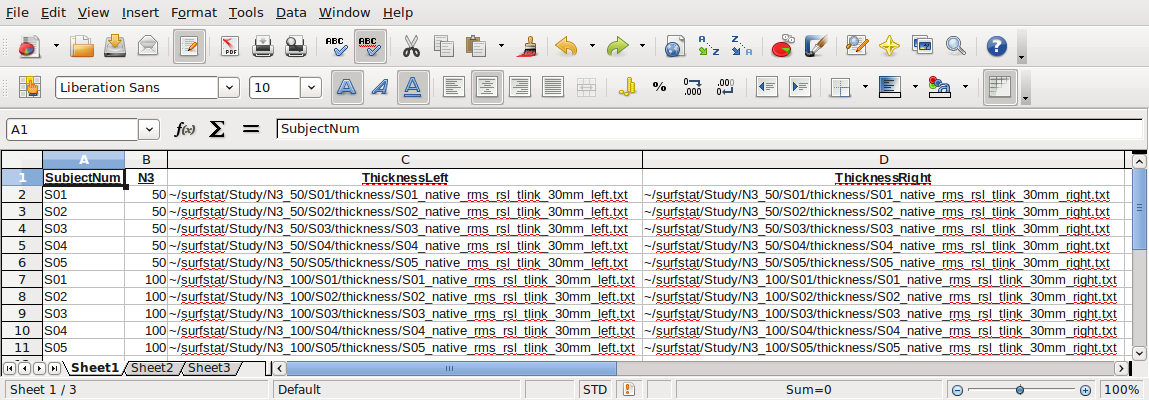
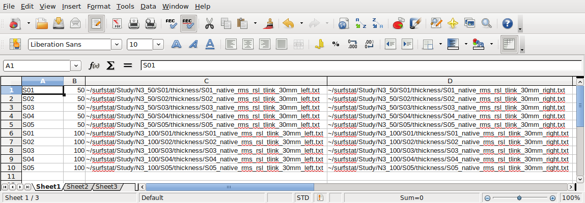
The headers at the top are beneficial for our learning purposes here (and you can save such a file for your own records, “glimfile_headers.csv”), but before use with Surfstat you will need to save a version without headers, “glimfile.csv”:

Your glimfile(s) should be located here:

MATLAB code: Surfstat Images

Sample MATLAB code can be found here in its entirety: N3 example. You may save it as a .m file. Hints for common parts that you are likely to need to edit are below:

%Creating the matrix of data.
[SubjectNum, n3, ThickFileLeft, ThickFileRight]=textread('glimfile.csv', ' %s %s %s %s');

• The variable names in square brackets should be in identical order as the columns in your glimfile.
• You will need to change the filename of the *.csv file to match the one you create.
• The number of %s (or %f in the case of continuous factors such as age) should be identical to the number of columns.
• It is recommended to use a lowercase first letter for “n3” in order to differentiate it from the capitalized “term” that we will create later on.

%Create terms
N3 = term (n3);

• You will need to create a “term” version of each variable in your model. Give it the same name as your variable, but capitalize it so you can tell them apart.

%% 1 You are now ready to create your model and to estimate it

Y = 1 + N3 + random(SubjectNum) + I;

• The linear model generally takes the form “Y = 1 + Variable1 + Variable2 …” and also includes the term “+ random(SubjectNum) + I” if any variables are within-subjects/repeated-measures. Since our current N3 analysis is simply two different parameters on the same subjects’ data, it is treated as a repeated measure. For more information: http://www.math.mcgill.ca/keith/surfstat/#mixed

%To get your t statistic for group
contrast_direction1 = N3.50 - N3.100;

• You can define a contrast by subtracting two levels of any term.
• The term name is before the period, and each level of it is after the period (and will be identical to whatever you called it in the glimfile). If you have any doubts about what the contrast levels are named, you can type the name of the term at the MATLAB prompt, and you will see the contrast level names as column headers.

%SurfStatColLim([-12,12]);

• This command sets the t map scale maximum and minimum values. It is currently commented out, as we recommend that you not use it during the first run. Let the scale set itself automatically so that you can get a better feel for the range of the values. Then, you may run it again, and select symmetrical min and max values of your choosing.

%To get your t statistic for group
contrast_direction2 = N3.100 - N3.50;

• Defining the contrast in the reverse direction is redundant for tmaps (it will just reverse the color scheme), but is necessary for viewing RFT (Random Field Theory) or FDR (False Discovery Rate) maps of any negative effects.

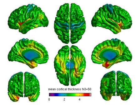
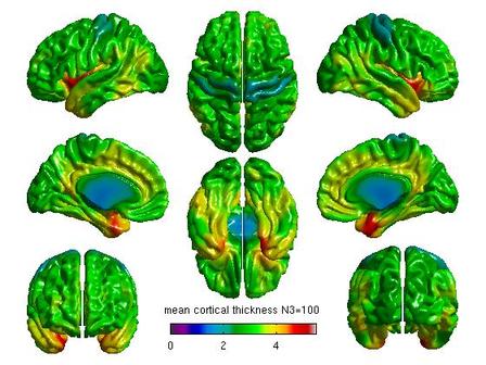
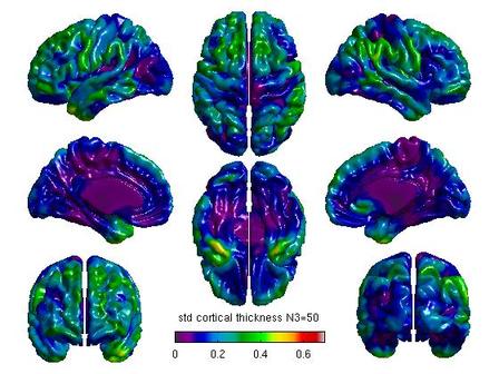
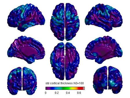
%Mean cortical thickness by N3
figure(6)
SurfStatView( mean(T3(1:5,:)), surf, 'mean cortical thickness N3=50');
set(gcf,'numbertitle','off','name','mean cortical thickness N3=50')
SurfStatColLim([0,5.5]);

figure(7)
SurfStatView( mean(T3(6:10,:)), surf, 'mean cortical thickness N3=100');
set(gcf,'numbertitle','off','name','mean cortical thickness N3=100')
SurfStatColLim([0,5.5]);

%Standard deviation by N3
figure(8)
SurfStatView( std(T3(1:5,:)), surf, 'std cortical thickness N3=50');
set(gcf,'numbertitle','off','name','std cortical thickness N3=50')
SurfStatColLim([0,.7]);

figure(9)
SurfStatView( std(T3(6:10,:)), surf, 'std cortical thickness N3=100');
set(gcf,'numbertitle','off','name','std cortical thickness N3=100')
SurfStatColLim([0,.7]);

• You can calculate a variety of other measures using SurfStatView, including mean and standard deviation of cortical thickness.

Output images

For each pair of N3 values that you wish to compare, you will need to create separate glimfiles, and run and modify this script. Example output images of N3=50 vs. N3=100 are below:

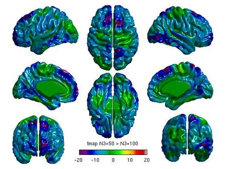
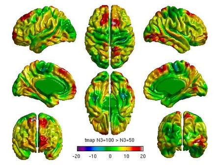
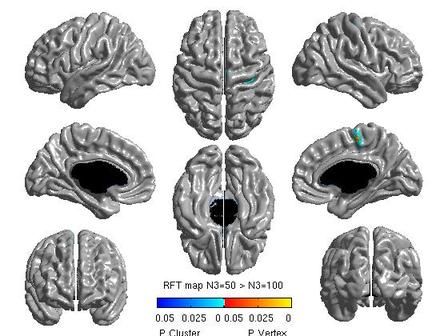
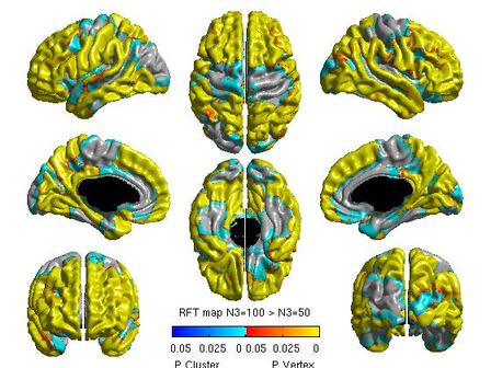
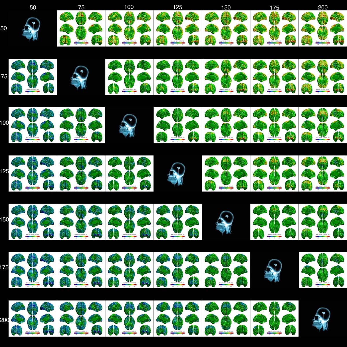
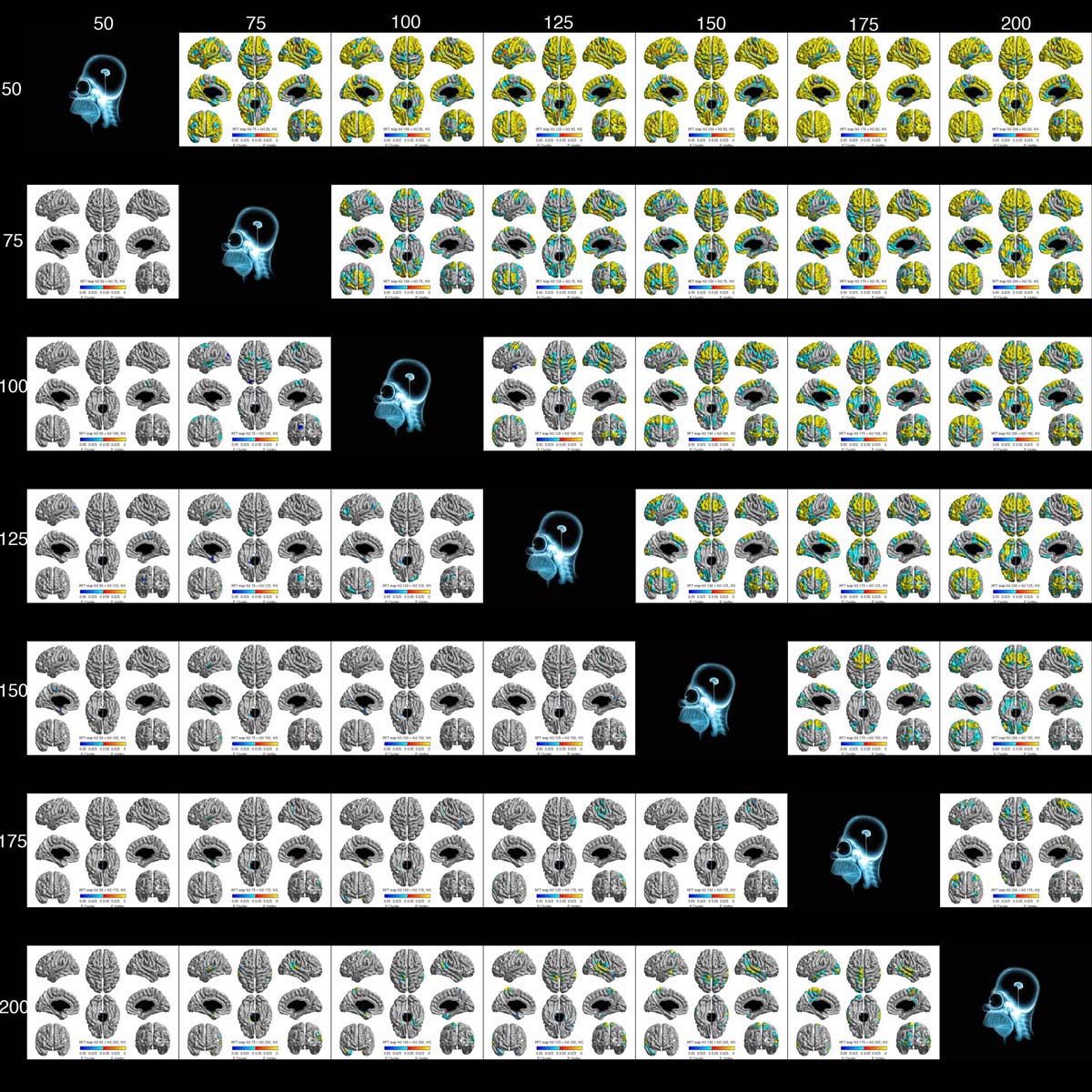
All pairwise comparisons can be combined into a montage of t or RFT maps:

MATLAB code: Plot Mean Cortical Thickness as a function of N3

Each time you run a pairwise comparison of N3 values, you can save the thickness values separated out for each N3. You will need to temporarily comment-out (or delete) the “clear” line:

%clear all; close all; clc

In the example in the section above, after the script is run, you would type in the MATLAB command prompt:

T3_50=(T3(1:5,:));
T3_100=(T3(6:10,:));

Next, rerun the script for all other N3 values, e.g., N3=75 vs. N3=125

T3_75=(T3(1:5,:));
T3_125=(T3(6:10,:));

And so on until you have run all N3 values. You may then save all of these values to a single .mat file:

save('N3.mat', 'T3_50', 'T3_75', 'T3_100', 'T3_125', 'T3_150', 'T3_175', 'T3_200')

This .mat file may be used to plot the mean and standard error of cortical thickness as a function of N3 value:

clear all
load N3.mat

Table_tlink = [mean(T3_50')' mean(T3_75')' mean(T3_100')' mean(T3_125')' mean(T3_150')' mean(T3_175')' mean(T3_200')'];
se_tlink = std(Table_tlink)'/sqrt(length(Table_tlink));

figure(1)

plot(mean(Table_tlink), 'ro-')
set(gca, 'XTick',1:7, 'XTickLabel',{'50' '75' '100' '125' '150' '175' '200'})
hold on
errorbar(mean(Table_tlink),se_tlink, 'r') %standard error
ylabel('Mean Cortical Thickness');
xlabel('N3');
set(gcf,'numbertitle','off','name', ['Mean Cortical Thickness as a function of N3']);

figure(2)

plot(se_tlink, 'ro-')
set(gca, 'XTick',1:7, 'XTickLabel',{'50' '75' '100' '125' '150' '175' '200'})
hold on
ylabel('Standard Error of Cortical Thickness');
xlabel('N3');
set(gcf,'numbertitle','off','name', ['Standard Error of Cortical Thickness as a function of N3']);

Output:

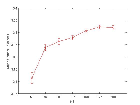
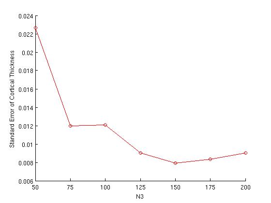
The plot on the right is simply a replot of the error bars from the plot on the left; at this scale, it is easier to see the N3 value at which variance is minimized (in this example, N3=150).

CIVET Home