 |
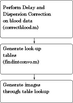
The diagram in figure 1 shows the general flow of performing rCBF analysis using MATLAB. First, the blood data is prepared for analysis by performing delay and dispersion correction. Next the lookup tables used in the analysis are calculated. Finally, the actual images are generated through table lookup using the lookup tables computed in the previous step.
Of course, the actual program implementation is slightly more complex than this. Figure 2 shows the full structure of the rcbf2 MATLAB function, which performs a full two-compartment rCBF analysis. All of the main functions that are called by rcbf2 are shown. The resampleblood function returns the blood data to rcbf2 in an evenly sampled time domain (sampled every 1/2second). This blood data is then passed to correctblood, which performs dispersion correction, and then delay correction by calling fit_b_curve. Finally, useful lookup tables are calculated by findintconvo.