SurfStat Analyses with CIVET
CIVET output may be used as input to Surfstat in order to conduct cortical thickness analyses. Here, we will walk you through a few simple examples of a between-subjects design, a within-subjects / repeated measures design, and a mixed design.
The purpose of this SurfStat documentation is to be a “quick start” guide, containing just the basic steps they are most likely to need to know. For more exhaustive documentation, we suggest you refer to:
(1) Setup
(2) Directory Structure
(3) Create a “glimfile”
(4) Using SurfStat in MATLAB
→ (4a) Load in data
→ (4b) Create terms
→ (4c) Visualize thickness: means and standard deviations
→ (4d) Create a general linear model (GLM)
→ (4e) Visualize thickness: t statistics, RFT, and FDR
→ (4f) Plotting data
(1) Setup
Required installations
- MATLAB: http://www.mathworks.com/products/matlab/ (We suggest an older version to optimize compatibility with SurfStat, e.g. R011b)
- Surfstat:
Required files
- Download CIVET average surfaces on which to display your group data here: CIVET_2.0.tar.gz, which contains:
CIVET_2.0_icbm_avg_mid_sym_mc_left.obj and CIVET_2.0_icbm_avg_mid_sym_mc_right.obj (for default / lores data, or you may also downsample hires data to this by taking data for only the first 40,962 vertices of each hemisphere)
CIVET_2.0_icbm_avg_mid_sym_mc_left_hires.obj and CIVET_2.0_icbm_avg_mid_sym_mc_right_hires.obj (for hires data)
CIVET_2.0_mask_left.txt and CIVET_2.0_mask_right.txt (hires, but can be downsampled to lores by taking data for only the first 40,962 vertices of each hemisphere)
CIVET_2.0_lobes_left.txt and CIVET_2.0_lobes_right.txt (hires, but can be downsampled to lores by taking data for only the first 40,962 vertices of each hemisphere)
CIVET_2.0_AAL_left.txt and CIVET_2.0_AAL_right.txt (hires, but can be downsampled to lores by taking data for only the first 40,962 vertices of each hemisphere)
CIVET_2.0_DKT_left.txt and CIVET_2.0_DKT_right.txt (hires, but can be downsampled to lores by taking data for only the first 40,962 vertices of each hemisphere)
- Or you may use an average surface of your own in .obj format (e.g., created using SurfStat tools to average mid resampled surfaces of all your subjects), but it’s not recommended.
- If you need an average surface / masks for CIVET 1.12 or earlier, you may find them here: CIVET_1.12.tar.gz
- Read this Sample MATLAB code to learn how to load the specific surfaces and masks for the model that you want to use. It’s important to know that the models for CIVET-1.X.Y and CIVET-2.0.0 are incompatible with one another and that you must load the appropriate model based on the version of CIVET that you used for your analysis. The default model in the current version of SurfStat (2015) is based on CIVET-1.
This tutorial assumes that you have already downloaded your data from CBRAIN. If you have not, please see the SFTP section to learn how to download your data.
(2) Directory structure
Create a directory in your home directory called “surfstat,” and within “surfstat” a subdirectory called “glimfiles.”
mkdir -p ~/surfstat/glimfiles
Make sure that your average surface(s), downloaded from CIVET_2.0.tar.gz, are in your surfstat folder:
ls ~/surfstat/CIVET_2.0_icbm_avg_mid_sym_mc_left.obj ls ~/surfstat/CIVET_2.0_icbm_avg_mid_sym_mc_right.obj
Make sure that the data you have downloaded from CBRAIN is in your surfstat folder:
ls ~/surfstat/<StudyName>
(3) Create a “glimfile”
The glimfile is a spreadsheet file (ending in .csv, space delimiters) that contains all of your study information to be read into Surfstat. Each row is a subject.
If you had run QC on your CIVET runs, within your study’s folder you will find a subdirectory called QC, and within that you will find a .csv file to get you started:
ls ~/surfstat/<StudyName>/QC/civet_<prefix>.csv
If you have not run QC, you can either go back and run it, or you can manually construct or script a glimfile yourself (space-delimited).
In this example, we use:
ls ~/surfstat/TETRIS/Time1/QC/civet_tetris.csv
and
ls ~/surfstat/TETRIS/Time2/QC/civet_tetris.csv
Where Time1 and Time2 are organized as 2 different CIVET studies with an identical set of subjects, one from Time1 and the other from Time2. Your data may be organized differently, but you will need to be consistent with its particular directory structures in the following steps.
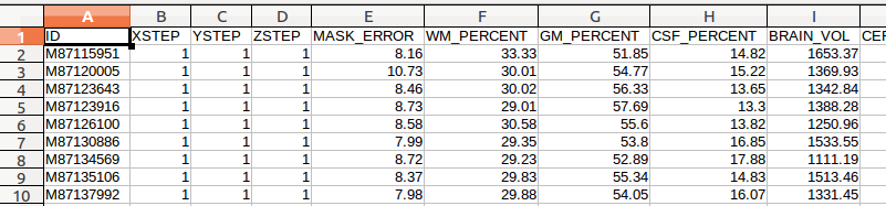
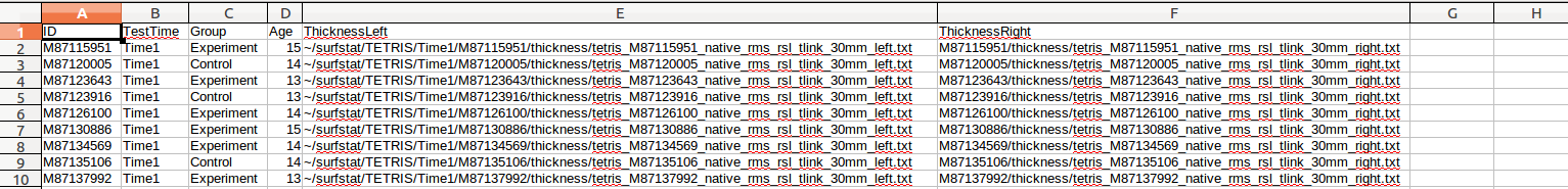
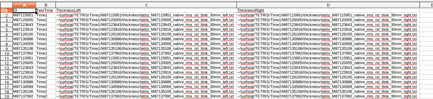
If you are able and interested in scripting the following process of setting up the glimfile, you may do so. We have provided sample MATLAB code to create a glimfile: MakeGlimFile_generic.m. Or, if you are not comfortable with programming, you may try the following. These files are comma-delimited, and can be opened for easy viewing in Excel, OpenOffice, etc. First, we look at ~/surfstat/TETRIS/Time1/QC/civet_tetris.csv:
Please note that even though you are opening it as comma-delimited, once you edit it you will need to save it as SPACE-delimited in order for the formatting to be compatible with SurfStat.
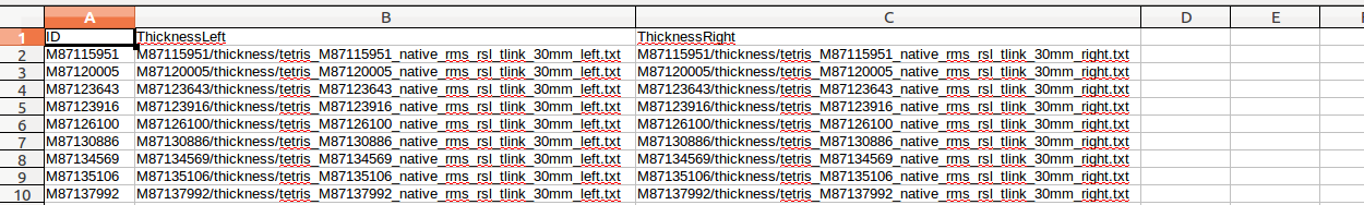
(A) There are many columns of data, and most of these you will not need. In this example, we only care about ID, ThicknessLeft and ThicknessRight (these are currently missing headers - to be fixed), so we delete all the other columns:
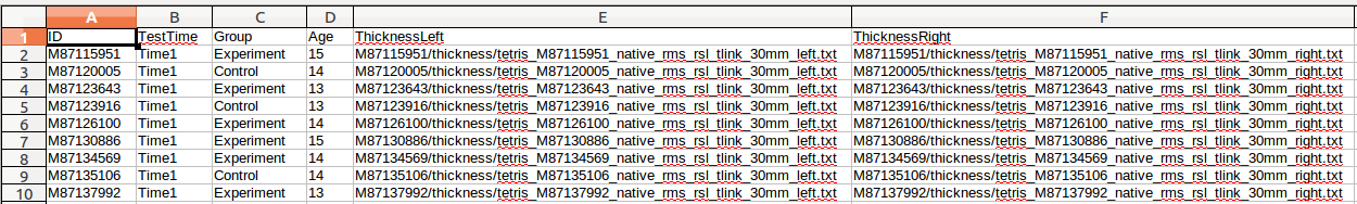
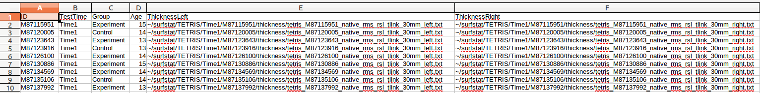
This example is a mixed design, because it contains a within-subjects / repeated measures variable (TestTime: Time1 vs. Time2) as well as between-subjects variables (Group: Experiment vs. Control; Age: continuous variable).
(B) Next, we are going to insert columns for our variables: TestTime, Group, Age:
For ThicknessLeft and ThicknessRight, we also need to be careful about designating exactly where our files are located. The .csv file output by CIVET QC contains a relative path, and not an absolute path. Note: Depending on your data organization and if you run your surfstat code directly from the surfstat directory, you may not need steps (C)-(F), i.e. if you are careful to load in your glimfile data from ~/surfstat/<Study> and if the first subject folder (<ID>) named in ThicknessLeft and ThicknessRight is located directly in ~/surfstat/<Study>/<ID> . In this example, the files listed are contained within the folder ~/surfstat/TETRIS/Time1/. To be safe, we create an absolute path by prepending ThicknessLeft and ThicknessRight with this for every row. This can be done manually, by scripting, or by the following little trick in OpenOffice:
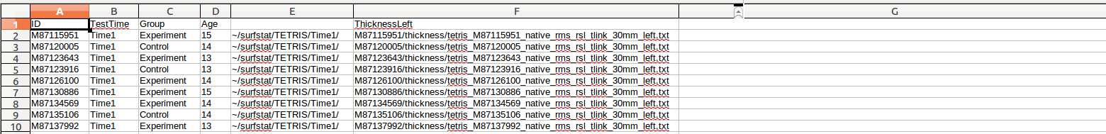
(C) First, insert 2 temporary new columns, 1 before ThicknessLeft, and 1 after ThicknessLeft. In the first entry of the 1st new column, enter ~/surfstat/TETRIS/Time1/, and copy/paste it for every row:
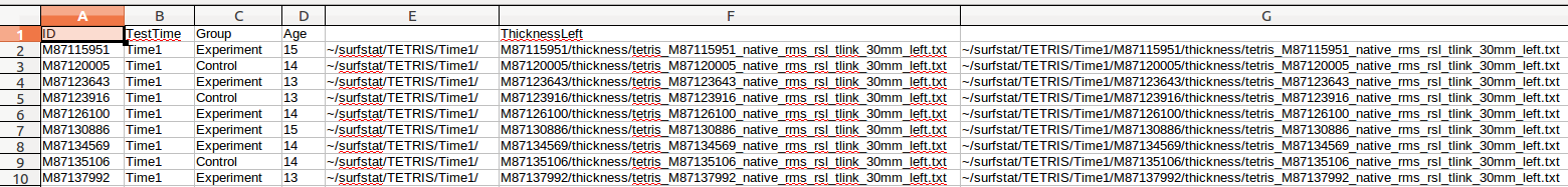
(D) Then, in the first entry of the 2nd new column (Column G here), enter =CONCATENATE(E2,F2) (where E2 and F2 are the immediately 2 preceding columns in the same row), and copy/paste it for every row:
(E) Now, we want to delete those 2 preceding columns. But if we were to do that right away, it would corrupt our concatenated column, which depends upon them. So we (1) copy all the values of the concatenated column, (2) select all the values from the ThicknessLeft column, (3) Right-click and select “Paste Special”, and (4) for “Paste Special” options, Select only Text. We have replaced our incomplete directories of ThicknessLeft with the full directory structure. Now we can delete those 2 extra rows that we had temporarily put in:
(F) Repeat for ThicknessRight, or simply copy/paste from ThicknessLeft and then find/replace all instances in that column of “left” with “right”:
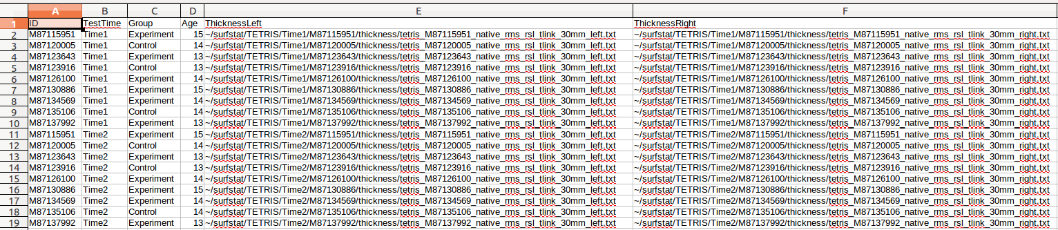
(G) We can now either repeat the above steps for ~/surfstat/TETRIS/Time2/QC/civet_tetris.csv, and then append it to the current file, OR simply (1) copy/paste everything into another simple. csv file, (2) find/replace all instances of “Time1” with “Time2”, and (3) append it the current file:
(H) We are going to save this file 2 ways. Save it with the headers, as:
~/surfstat/glimfiles/<StudyName>_glim_headers.csv (here, we use ~/surfstat/glimfiles/tetris_glim_headers.csv)
(I) Then delete just the first row (the headers only), and save again (space-delimited, not comma-delimited!) as
~/surfstat/glimfiles/<StudyName>_glim.csv (here, we use ~/surfstat/glimfiles/tetris_glim.csv)
The version with the headers is for your future reference, but the one without headers is the one that SurfStat can read.
Tip: if you ever have problems with opening a glimfile in SurfStat, try opening it in a simple text viewer (TextEdit, WordPad, vi, etc.) and confirm that it is indeed space-delimited. If you run into problems with commas, you can also simply use the following Unix command to replace all commands in your glimfile with spaces:
sed ‘s/,/ /g’ ~/surfstat/glimfiles/tetris_glim.csv > ~/surfstat/glimfiles/tetris_glim2.csvmv ~/surfstat/glimfiles/tetris_glim2.csv ~/surfstat/glimfiles/tetris_glim.csv
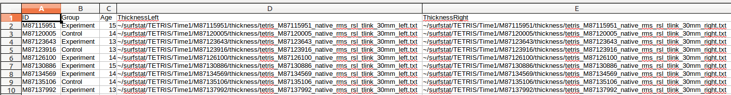
We chose this example as a relatively complex design (mixed-design, containing both between- and within-subject variables) in order to show you the most complex scenario. However here are contrasting examples of glimfile construction if this were only a between-subjects design:
vs. if this were only a within-subjects design (whenever there is a repeated-measure, there will be TWO ROWS per subject ID):
(4) Using SurfStat in MATLAB
Sample MATLAB code can be found here in its entirety: Sample MATLAB code. You should copy/paste and save it as a .m file. Hints for common parts that you are likely to need to edit are below:
(4a) Load in data
%Creating the matrix of data.
[id, testtime, group, age, ThickFileLeft, ThickFileRight]=textread('/home/llewis/surfstat/glimfiles/tetris_glim.csv', ' %s %s %s %f %s %s');   %textread does not understand ~, so type in your entire path
- The variable names in square brackets should be in identical order as the columns in your glimfile.
- You will need to change the filename of the *.csv file to match the one you create.
- The number of %s (or %f in the case of continuous factors such as age) should be identical to the number of columns.
- It is recommended to use a lowercase first letter for variables in order to differentiate them from the capitalized “term” that we will create later on.
(4b) Create terms
%Create terms
TestTime = term (testtime);
Group = term (group);
Age = term (age);
- You will need to create a “term” version of each variable in your model. Give it the same name as your variable, but capitalize it so you can tell them apart.
(4c) Visualize thickness: means and standard deviations
%% MEANS & STDS
%Mean cortical thickness for all
figure
SurfStatView( mean(T3).*mask, surf, 'mean cortical thickness');
SurfStatColLim([0.5,5.5]);

%Standard deviation of cortical thickness for all
figure(
SurfStatView( std(T3).*mask, surf, 'std cortical thickness');
SurfStatColLim([0,.7]);
- First, we take a simple look at the mean and standard deviation maps across all data. The commands above produce:

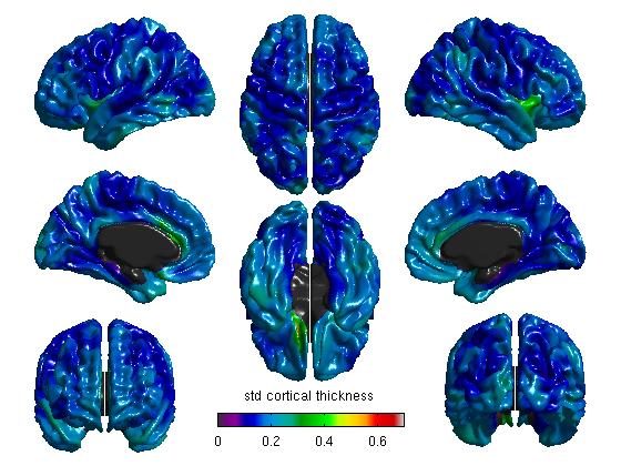
Hint: as a sanity check, you may also do this without the midline mask (remove “.*mask” from the commands above). You should see the data clearly outlining the midline. If it looks off-center, it is possible that (A) you mixed up CIVET 1.11 or CIVET 1.12 data with the CIVET 2.0 average surface, or vice versa, or (B) if you scripted it yourself, that you used non-resampled (native) data on the average surface.
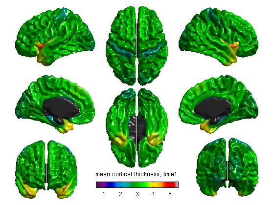
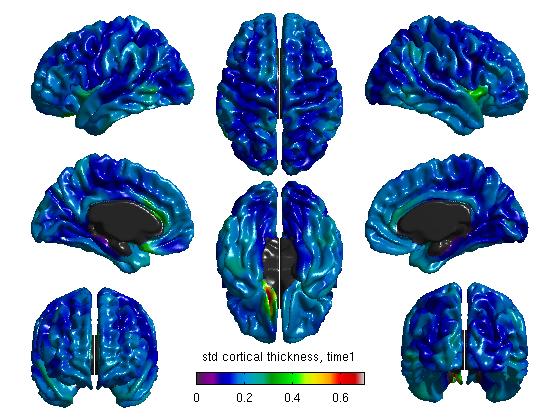
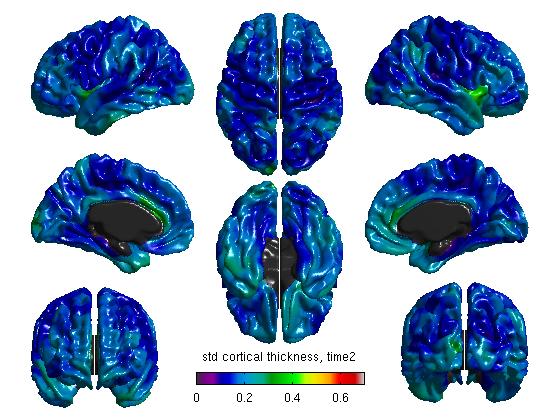
%Mean cortical thickness, per TestTime
figure
SurfStatView( mean(T3(1:27,:)).*mask, surf, 'mean cortical thickness, time1');
SurfStatColLim([0.5,5.5]);

figure
SurfStatView( mean(T3(28:54,:)).*mask, surf, 'mean cortical thickness, time2');
SurfStatColLim([0.5,5.5]);

%Standard deviation of cortical thickness, per TestTime
figure
SurfStatView( std(T3(1:27,:)).*mask, surf, 'std cortical thickness, time1');
SurfStatColLim([0,.7]);

figure
SurfStatView( std(T3(28:54,:)).*mask, surf, 'std cortical thickness, time2');
SurfStatColLim([0,.7]);
- We can also separate our data by the top 27 rows (Time1) and the bottom 27 rows (Time2). Of course, these numbers will vary depending on your number of subjects. The commands above produce:

(4d) Create a general linear model (GLM)
%% 1 You are now ready to create your model and to estimate it

Y = 1 + TestTime + Group + Age + random(id) + I;
slm = SurfStatLinMod( T3, Y, surf );
- The linear model generally takes the form “Y = 1 + Variable1 + Variable2 …” and also includes the term “+ random(id) + I” if any variables are within-subjects/repeated-measures. For more information: http://www.math.mcgill.ca/keith/surfstat/#mixed
(4e) Visualize thickness: t statistics, RFT, and FDR
%% MAIN EFFECT OF GROUP, DIRECTION 1 (EXPERIMENT > CONTROL)

%To get your t statistic for group
contrast_group_direction1 = Group.Experiment - Group.Control;
slm_group_direction1 = SurfStatT ( slm, contrast_group_direction1);
figure(2)
SurfStatView ( slm_group_direction1.t.*mask, surf, 'tmap exp>cont, removing age, test-time' );
- You can define a contrast by subtracting two levels of any discrete term (such as Group). This variable is then plugged in as the second argument of SurfStatT. For continuous factors (such as age), please see below.
- The term name is before the period, and each level of it is after the period (and will be identical to whatever you called it in the glimfile). If you have any doubts about what the contrast levels are named, you can type the name of the term at the MATLAB prompt, and you will see the contrast level names as column headers.
- Any variable that is included in the linear model equation (Y = 1 + …) but is not included in a particular contrast is removed/controlled for in that contrast.
%SurfStatColLim([-3,3]);
- This command sets the t map scale maximum and minimum values. It is currently commented out, as we recommend that you not use it during the first run. Let the scale set itself automatically so that you can get a better feel for the range of the values. Then, you may run it again, and select symmetrical min and max values of your choosing.
%To get thresholded p values using Random Field Theory
[ pval, peak, clus ] = SurfStatP( slm_group_direction1, mask );
figure
SurfStatView( pval, surf, 'RFT exp>cont, removing age, test-time');
%To get thresholded p values using False Discovery Rate
qval = SurfStatQ( slm_group_direction1, mask );
figure
SurfStatView( qval, surf, 'FDR exp>cont, removing age, test-time');
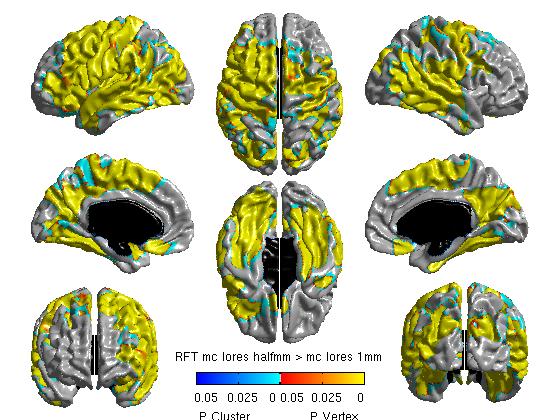
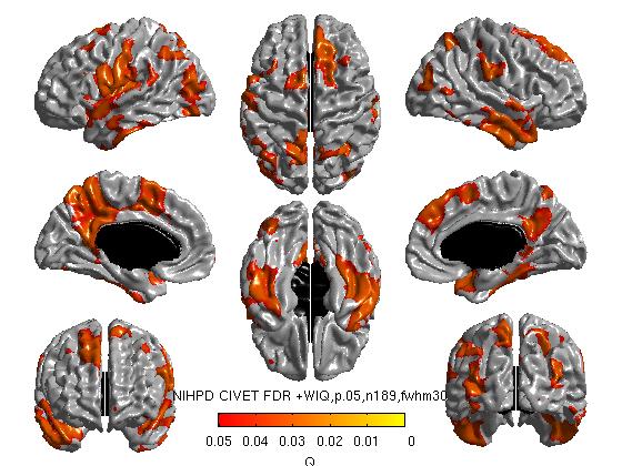
- The 3 commands above produce t stat maps, RFT and FDR maps, respectively. RFT maps (strict) and FDR maps (a bit less strict) assess statistical significance accounting for multiple comparisons:
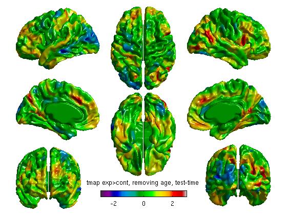


Our own FDR and RFT maps in this example are blank (showing no areas of statistical significance), perhaps due to small n size with this sample experiment. As a quick aside, here are 2 examples of significant FDR and RFT maps from other studies: RFT.jpg and FDR.jpg
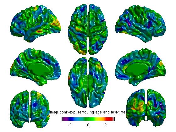
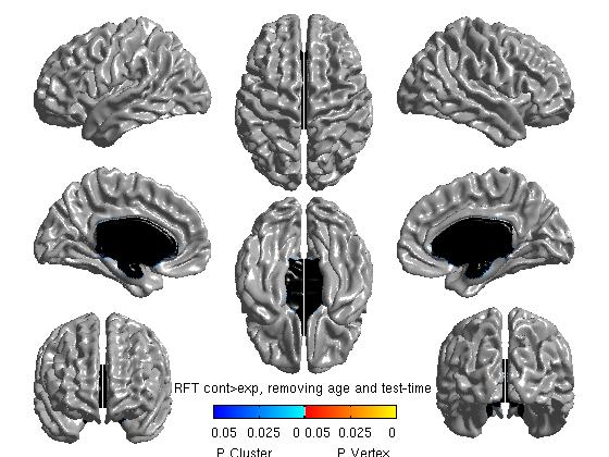
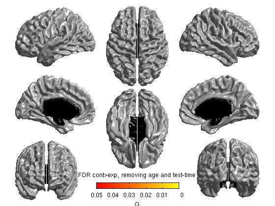
% MAIN EFFECT OF GROUP, DIRECTION 2 (CONTROL > EXPERIMENT)

%To get your t statistic for group
contrast_group_direction2 = Group.Control - Group.Experiment;
slm_group_direction2 = SurfStatT ( slm, contrast_group_direction2);
figure
SurfStatView ( slm_group_direction2.t.*mask, surf, 'tmap cont>exp, removing age and test-time' );
SurfStatColLim([-3,3]);
%%To get thresholded p values using Random Field Theory
[ pval, peak, clus ] = SurfStatP( slm_group_direction2, mask );
figure
SurfStatView( pval, surf, 'RFT cont>exp, removing age and test-time');
%%To get thresholded p values using False Discovery Rate
qval = SurfStatQ( slm_group_direction2, mask );
figure
SurfStatView( qval, surf, 'FDR cont>exp, removing age and test-time');
- Defining the contrast in the reverse direction is redundant for tmaps (it will just reverse the color scheme), but is necessary for viewing RFT (Random Field Theory) or FDR (False Discovery Rate) maps of any negative effects. The commands above yield the following figures:
Note: the default threshold for RFT is 0.001 and for FDR is 0.05. The RFT one is extremely strict, and Boris Bernhardt and Keith Worsley have suggested that it may be loosened to 0.01, maybe up to to 0.025. To change them:
%% EXAMPLES OF HOW TO CHANGE THE RFT OR FDR THRESHOLD

%%To get thresholded p values using Random Field Theory
p='0.02'; %choose your threshold different from 0.01
[ pval, peak, clus ] = SurfStatP( slm_group_direction2, mask, str2num(p) );
figure
SurfStatView( pval, surf, ['RFT cont>exp, p<' p]);
%%To get thresholded p values using False Discovery Rate
p='0.02'; %choose your threshold different from 0.05
qval = SurfStatQ( slm_group_direction2, mask );
figure
SurfStatView( qval, surf, ['FDR cont>exp, p<' p] );
For an example of how to analyze age, see the Age example on Keith Worsley’s page.
(4f) Plotting data
There are a variety of simple plotting examples using SurfStatPlot on Keith Worsley’s page.
However, you may also use MATLAB’s functionality. If you wish to collapse values across vertices, it is critical to first exclude the vertices that fall under the midline mask:
%T3_masked=T3(:,find(mask)); %exclude masked vertices
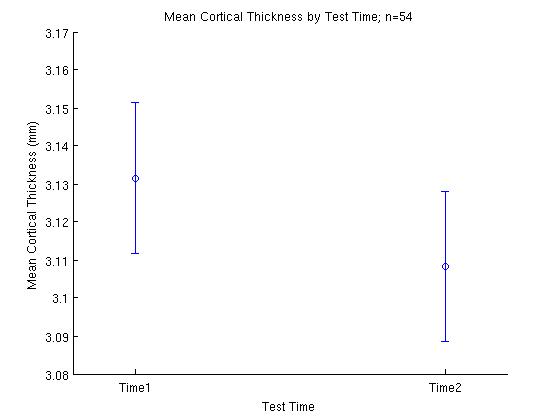
Imagine that you wish to show the mean and standard error thickness across subjects:
subj_means_collapsed_across_vertices= mean(T3_masked');
means=[mean(subj_means_collapsed_across_vertices(1:27)), mean(subj_means_collapsed_across_vertices(28:54))];
standarderror=[(std(subj_means_collapsed_across_vertices(1:27))/sqrt(length((subj_means_collapsed_across_vertices(1:27))))), ...
               (std(subj_means_collapsed_across_vertices(28:54))/sqrt(length((subj_means_collapsed_across_vertices(28:54)))))];
figure
hold on
plot(means, 'bo');  %b is for blue and o is for the marker, you can play with these options
set(gca, 'XTick',1:2, 'XTickLabel',{'Time1' 'Time2'})
errorbar(means,standarderror, 'bo') %standard error

ylabel('Mean Cortical Thickness (mm)');
xlabel('Test Time');
title (['Mean Cortical Thickness by Test Time; n=' num2str(length((subj_means_collapsed_across_vertices)))]);
The code above produces:
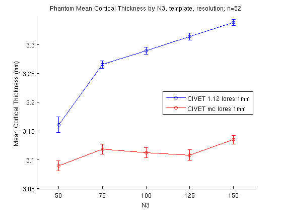
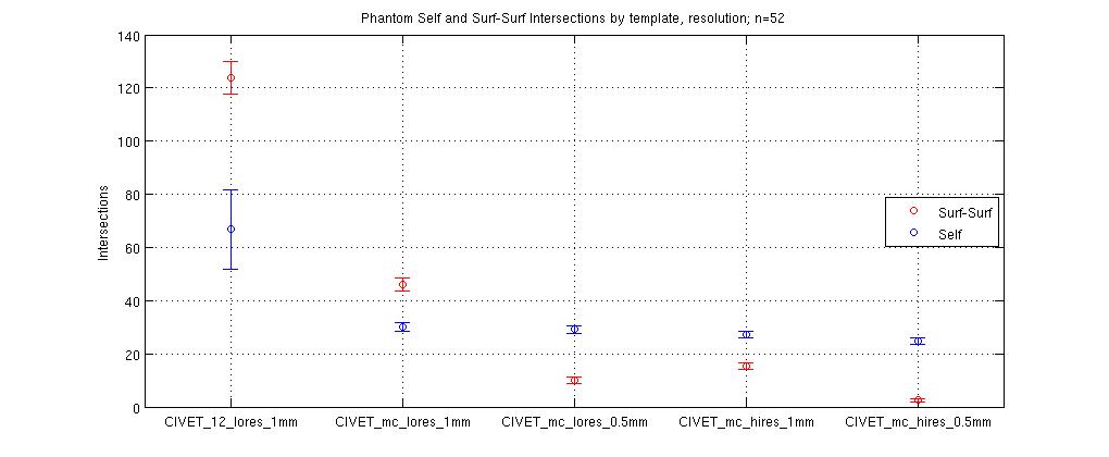
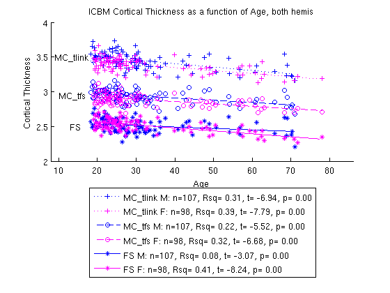
A few more examples of figures produced by MATLAB: