Transcranial Magnetic Stimulator
The 3-Dimensional Mapping of the Magnetic Field
 
Apparatus and Set-Up

Theoretical Predictions


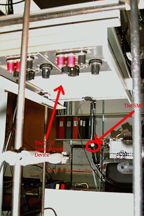
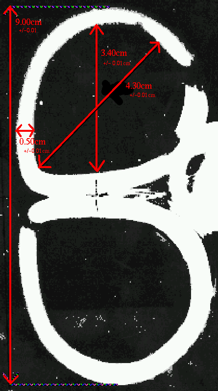
Figure 5:  An x-ray image of the two lobed TMS coil 
(Click image to view enlarged version)


Figure 6:  A blackened image of one lobe of the TMS coil used for the input of the programs for the theoretical model

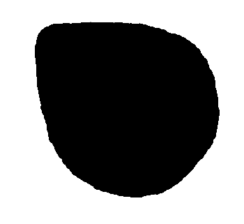
    Figure 5 depicts and x-ray image of the figure-of-eight coil which was studied in this laboratory.  The determination of an generalized equation that describes the magnetic field around the coil under investigation was required to do the theoretical predictions.  To determine the magnetic field equation, the coil was split into infinitesimal line segments.  Given the two end points on the line segment and the point in space you wished to determine the field at, a generalized equation for the magnetic field was determined.  
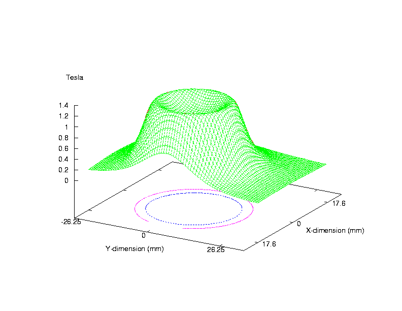
Equations 3,4,5,6,and 7 were used to determine the magnetic field of small line segments (on the coil) along one plane parallel to the coil for various points.


    The vector components of the calculated field at any particular point due to each line segment was then added together to get the total magnitude of the magnetic field.  Since this procedure would be quite difficult to complete by hand, a C program was written to perform the task.  The correct dimensions of the coil under investigation was determined by taking the x-ray image of the coil and scanning it into the computer at 300dpi.  Figure 5 depicts the x-ray image of the coil.  The TMS coil consists of two lobes, each of which is teardrop shaped.  Each lobe contains 14 windings of copper as determined by viewing the x-ray through a traveling microscope.  To allow the computer to draw a line image of the shape of the coil, a blackened image of one of the lobes was created by using a image editor such as gimp (on unix) shown in Figure 6.


    Figure 7 illustrates a schematic of the TMS coil and the orientation of the windings.  The coil itself is cooled with a steady stream of air since the TMS coil become very hot during repetitive prolonged use.

   The current travels in the same direction in the center of the TMS coil and in phase.  This was determined by using a magnetometer which is a digital hall probe.  A constant DC current of 2A were sent into the TMS coil and the hall probe was used to determine the direction of the magnetic field.  Once the direction of the magnetic field was determined, the direction of the current can be easily determined according to the right hand rule.  The coil itself is made of copper.

    The program used to determine the theoretical distribution of the magnetic field consisted of three components.  The initial component took the scanned solid image of the coil and determined its center of mass.  After finding the center of mass of the object, a function which related the radius and angle with respect to the center of mass was determined.  The output of this program produced an outline of the shape of the coil.  The second stage of the program took the outline and placed the coil in the orientation that the experimenter wished to study.  This part of the program only became important when the complete TMS coil was of interest.


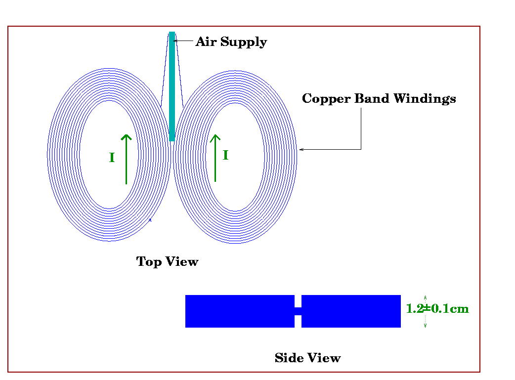
Figure 7:  Schematic of the TMS coil indicating the direction of the current
(Click image to view enlarged version)


Figure 8:  Theoretical 3-Dimensional Magnetic Field Distribution for a circular wire at a distance of 1.5cm above the wire

(Click image to view enlarged version)


     That is, a mirror image of the lobe could be made.  The final stage of the program did the actual calculations of the field.  To test the program, the theoretical field distribution for a circular wire was determined and is shown in Figure 8.

     The C programs that were created to produce the theoretical 3-dimensional distributions are included in Appendix II along with the necessary instructions for using them.

Experimental Measurement

    In order to measure the magnitude of the magnetic field generated by the TMS coil, a detection coil was constructed.  In order to ensure that contributions to the total flux from all three planes would be detected, three circular loops of copper were wound 6 times each around a plastic bead.Each loop was placed on the bead perpendicular to each other.  That is, each loop was strategically placed in the x, y and z planes. 

   Figure 9 illustrates the configuration of the pick up coil designed for this experiment.  The magnetic flux through the surface of each plane in the detection coil can be described by equation 9.

   With the flux, we then calculate the voltage induced by the TMS coil on the detection coil.  This is described by Faraday's Law on induction, as given in equation 10.


Figure 9:  The magnetic field pickup sphere (SMP)


Figure 10:  The general setup of the experimental collection of data

(Click image to view enlarged version)


   This voltage is recorded by the Labmaster and was used to map the magnetic field distribution.  The xy Translational Device was constructed out of a Hewlett-Packard XY plotter so that the SMP could be moved in the x and y direction in steps of 2.0mm.  The three dimensional induction coil was mounted on the xy translational device so that it is suppended in space above the TMS coil.  Figure 10 illustrates the schematic of the overall setup of the experiment.  Figure 11 illustrates the SMP mounted onto the xy translational device.


Figure 11:  The SMP mounted on the xy translational device as seen in the lab.
(Click image to view enlarged version)
   To control its movement, a Labmaster Digital/Analogue converter and a 486 computer was used.  Control.c was written to move the coil in a rectangular grid matching the dimensions of the TMS coil in steps 2.0mm in the x and y directions.  Once control.c had moved the detection coil to the desired position, the TMS coil was triggered to emit a magnetic pulse and the induced current on the SMP was inputted into a circuit which consisted of a half wave rectifier and an integrator as shown in Figure 12.  (control.c is included in Appendix II)  Three circuits of the type  shown is Figure 12 were required since there are three pick up coils for the x, y, and z components on the SMP.  Initially, the signal was seen on an oscilloscope with the use of a single coil loop.  Figure 13 depicts an illustration of the signal seen.  The peak to peak voltage is 50 +/- 1 mV and the period is 200 +/- 2s.

Figure 12:  The circuit used for the collection of data from the SMP.
(Click image to view enlarged version)


Figure 13:  A sketch of the signal seen on the oscilloscope


    This signal was then sent to the ADC of the Labmaster which was recorded by the computer.  A suitable interval time was chosen so that for each measurement of one point, it allowed for latent fields to dissipate from the system before moving onto the next point.  The time interval between measurements was determined to be 1.0 +/- 0.2s.  The peak current flowing through the coil was 3.6kA (Specified by the Manufacturer - Cadwell) and it flowed in opposite directions and in phase in the two lobes.  The experimental measurements were taken at 50 +/- 5% of the maximum power output of the Cadwell Stimulator.

 
Figure 14:  The coordinate designation of x and y with respect to the TMS coil.  The orientation of the SMP for each component is also shown.
    The designation of the x, y and z coordinate was chosen as shown in Figure 14.  The x component of the magnetic field was measured by the coil on the SMP in configuration A.  The y component was measured by the coil in configuration B and the z component is measured by the coil in configuration C.  This was arbitrarily set by the experimenter.  The measuring procedure started with the SMP positioned at point Q. The SMP then traversed in the y direction then reset to a point  where  is a step in the x direction.  is 2.0mm.  The SMP then continues to traverse in the y direction again.  This was repeated for 30 steps in both the x and y directions.

    A proper scaling of the step sizes was then completed.  In order to accomplish this, a pen was placed in place of the SMP and the position of the SMP for each step was mapped out on paper which corresponded to the TMS position.  Once this was known, the position of the SMP (in centimeters) was determined by re-scaling the step sizes to the actual dimensions of the coil.  The center of the TMS coil is shown in Figure 14 by the cross was designated as the origin (0cm, 0cm).


[Home] [Introduction] [Theory] [Apparatus and Set-Up] [Data and Results] [Conclusion] [Bibliography] [Appendix I] [Appendix II] [Acknowledgments]