2. Context in Image Classification
a. Lower Order Markov Chains3. Context in Text Recognition
b. Hilbert Space Filling Curves
c. Markov Meshes
d. Dependence Trees
a. A Quick Bit on Compound Decision Theory
b. Dictionary Look-up Methods
2. Context in Image Classification
d. Dependence Trees Chow
A dependence tree is used to apply a tree dependence to approximate probability distributions. A dependence tree indicates the dependence of pixels on other pixels.
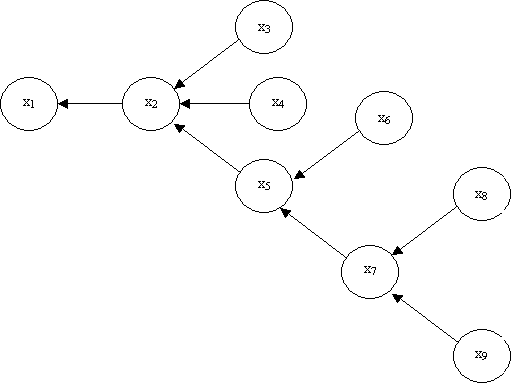
For example in the figure
above shows that for a pixel xk, which pixels are dependent
on the others. For example the pixel x2 is dependent on
pixel x1, and pixels x3, x4, and x5
are dependent on x2. As we did in Markov chains consider
the following, the joint probability distribution P(X) where X is
a vector of N discrete random variables ![]() .
In order to determine the probability distribution for a certain configuration
of X, an approximation can be used, which is the product of lower order
probability distributions. This is valid, because any product approximation
is also a valid probability distribution.
.
In order to determine the probability distribution for a certain configuration
of X, an approximation can be used, which is the product of lower order
probability distributions. This is valid, because any product approximation
is also a valid probability distribution.
Assume once again that we
have a predefined dependence tree for each class of object that we are
looking to define. This dependence tree method will help classify
images into there predefined classes.
Consider a probability distribution permissible as an approximation of the following form:
![]() .
.
M=![]() is
an unknown permutation of integers where at least on of the variables in
represented. The function j(i) is called the dependence tree of the
distribution and represents the mapping that is required in order to define
the dependence tree.
is
an unknown permutation of integers where at least on of the variables in
represented. The function j(i) is called the dependence tree of the
distribution and represents the mapping that is required in order to define
the dependence tree.
Let xi represent a
point in the plane that defines a point in the plane. Consider now
two variables xq and xp such that the
mapping function yields the result that p=j(q). Therefore
the dependency function has told us that xq is dependent
on xp. This is defined in the dependence tree graph
by an arrow pointing xq from to xq.
If
j(q)=0 the there will be no arrow pointing away from the variable
xq.
Optimum Approximation
In order to determine dependencies, an approximation of the form discussed above must be discussed. Consider again a probability distribution of n discrete variables, such that![]() and has the property that
and has the property that ![]() .
.
The mutual information between two probability distributions is defined as is the measure of closeness in approximating P by using the approximated distribution Pa. I(P, Pa) can be viewed as the difference in information content between the two probability distributions. The measure is always positive if the two distributions ae different and zero is they are the same. The mutual information is easily applied when the distribution is a product expansion. We will use this measure to define a approximating a probability distribution as a dependence tree.
We know that if we were to do an exhaustive search for a set of N variables, then there are a possibility of NN-2 with N vertices. Therefore for any reasonable value of N this would take an enormous amount of time therefore, we are better off approximating the distribution. Therefore for an Nth-order probability distribution, P, we wish to find the distribution of tree dependence Pa. LEt us first consider the following two definitions in order to aid with the optimization problem:
Definition 1:
The mutual information between two random variables xi and xj is defined as follows:
 .
.
If we use the mapping of j(i) then the mutual information between the random, ie: I(xi,xj) is variable and its mapping will be useful quantities.
Definition 2:
What we would like to define is a maximum weight dependence where each branch has the maximum possible weight that it can have. This means that the mutual information between xi and xj is a maximum. The probability distribution of tree distribution for a tree dependence Pt(X) is an optimum approximation to P(X) if and only if its dependence tree is of maximum weight.
If we expand ![]() using Pt(X) and P(X) as the functions which
we are trying to find the mutual information of we can expand the following:
using Pt(X) and P(X) as the functions which
we are trying to find the mutual information of we can expand the following:
 -----(*)
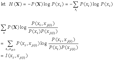
We can also define H(X) as the following as well as the mutual information function as the following.:

Now if we substitute into (*) we get the following to define our mutual information function:
![]() .
.
H(xi)
and H(X) are both independent of the dependence tree, and
I(P,Pt)
is non-negative, therefore if we are able to
minimize the closeness measure, or the mutual information function, then
we can maximize the branch weight ![]() .
.
Of course we don't want to search through every possibility of branch weight in order to figure out what the optimal tree is. Therefore we must use an optimization procedure.
Optimization Procedure
The problem is now to construct a dependence tree with maximum weights for each branch of the tree.
1) Read in samples of and
image ![]() from the
image to be classified.
from the
image to be classified.
2) Calculate the pairwise Mutual Information measures I(xi,.xj) must be directly evaluated
3) Find the maximum measure of the mutual information of the an make those the first nodes of the dependence trees. Keep adding branches as we know the maximum mutual information measures. The problem is to make the dependence tree of maximum total branch weight.
-order the branches from according to decreasing weights, where the weighting is the Pairwise Mutual Information measure presented aboveAn Example and an Animation
-for some branch bi is less than or equal to the weight for some branch bj where i<j
-select b1 and b2 and add b3 so that it does not form a cycle with b1 and b2
-unique solutions are possible if all the branch wieghts are different, but several solutions are possible if there are some weights that are the same
Consider the following probability distribution for four pixels:
The numbers here are fairly irrelevant, but what is most important, is to understand the procedure needed in order to create a dependence tree.
A Binary Probability Distribution
| x1x2x3x4 | P(x1x2x3x4) | P(x1)P(x2)P(x3)P(x4) |
| 0000 | 0.100 | 0.046 |
| 0001 | 0.100 | 0.046 |
| 0010 | 0.050 | 0.056 |
| 0011 | 0.050 | 0.056 |
| 0100 | 0.000 | 0.056 |
| 0101 | 0.000 | 0.056 |
| 0110 | 0.100 | 0.068 |
| 0111 | 0.050 | 0.068 |
| 1000 | 0.050 | 0.056 |
| 1001 | 0.100 | 0.056 |
| 1010 | 0.000 | 0.068 |
| 1011 | 0.000 | 0.068 |
| 1100 | 0.050 | 0.068 |
| 1101 | 0.050 | 0.068 |
| 1110 | 0.150 | 0.083 |
| 1111 | 0.150 | 0.083 |
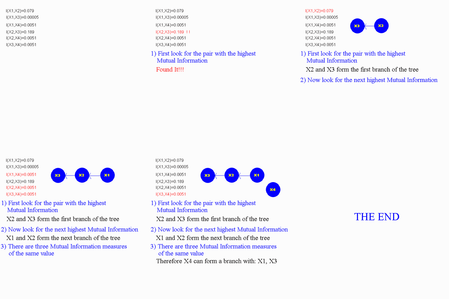
From this the following Pairwise Mutual Information values can be calculated:
I(x1,x2)=0.079
I(x1,x3)=0.00005
I(x1,x4)=0.0051
I(x2,x3)=0.189
I(x2,x4)=0.0051
I(x3,x4)=0.0051
The following animation will demonstrate how to construct a dependence tree.

Previous : 2b.Markov
Meshes
Next: 3.
Context in Text Recognition