2. Context in Image Classification
a. Lower Order Markov Chains3. Context in Text Recognition
b. Hilbert Space Filling Curves
c. Markov Meshes
d. Dependence Trees
a. A Quick Bit on Compound Decision Theory
b. Dictionary Look-up Methods
2. Context in Image Classification
b. Hilbert Space Filling Curves Abend
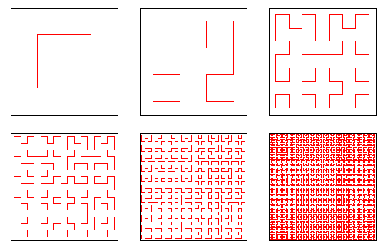
Now that the nearest neighbor dependence of Markov chains has been looked at, we need to look at a method which quickly and efficiently looks at every pixel within an image. The chain assumption presented in the Markov chains section can then be applied. What we would also looking to do is find a manner in which to traverse all the pixels such that we can apply the Markov Mesh analysis. The challenge is to scan the image using a continuous curve, which passes through every pixel on the pixel grid is as "crimpled" as possible. It also stands to reason that we would want our algorithm not to intersect over itself, thus making it run more efficiently.The curve scans a pixel array which has a size of 2m x 2m pixels. The curve scans the array while never maintaining the same direction for more than three consecutive points. Once the curve has strayed three points in a straight line it turns around and comes back. When the curve "turns around" it turns right (with respect to the direction that it is facing) and moves to the next pixel and turns right again and starts heading back towards
 http://www.math.ohio-state.edu/~fiedorow/math655/Peano.html
An Algorithm to Define Hilbert Sapce Filling
Curves http://www.cut-the-knot.com/do_you_know/hilbert.shtml
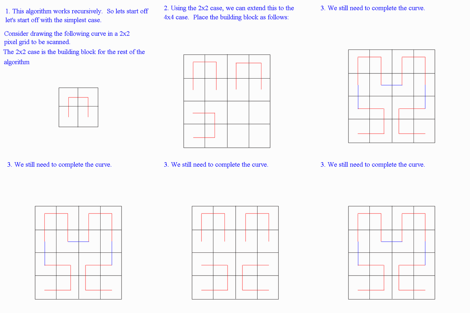
Below there is an animation
which describes how the algorithm works. Essentially one can see
that the algorithm is recursive and can be used repeatedly to create curves
which are continuous and non intersecting such that every pixel in a grid
is traversed once, and only once.
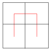
First start with the following "element" of the Hilbert Space filling curve. This will be like a building block for the rest of the curve.

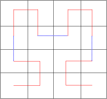
If we then consider how to
make a space filling curve in a 8 x 8 grid, we use this building block
again. We put a translation of this unit in the two top corners and
then rotate them by a 90 degrees clockwise and counter clockwise so that
they can be placed in the bottom two corners of the pixel grid. The
dotted blue lines indicate how to connect the elements of the Hilbert Space
filling curves.

The following animation shows how the algorithm works.

This can easily be extended to any 2mx2m case by filling the grid with the result above and by looking at the grid in subgroups of 4x4 pixels.
The curve has some really
nice properties. It can scan an array of 2m x 2m
array of pixels while never maintaining the same direction for more
than three consecutive pixels. After the curve moves by three pixels,
it turns around and come back without ever having to visit the same pixel
more than once. However we must now take a look at how the spatial
dependencies can affect the classification of images, and for this we will
look at Markov meshes.
Previous : 2a.
Lower Order Markov Chains
Next: 2c.
Markov Meshes