The Use of Context in Pattern Recognition

1. Introduction

2. Context in Image Classification

a. Lower Order Markov Chains
b. Hilbert Space Filling Curves
c. Markov Meshes
d. Dependence Trees

a. A Quick Bit on Compound Decision Theory
b. Dictionary Look-up Methods

4. Conclusions

References

2.  Context in Image Classification

As was mentioned in Section 2a about Lower Order Markov Chains,  there is another project in this course that covers Markov Dependencies, therefore Markov meshes will not be covered in too much depth in this section of the project.  What will be discussed is primarily available in a paper by Abend et al.

We know already from the section on Lower Order Markov Chains, how a pixel behaves in a chain.  However we know that our images exist in a two dimensional array.  We have also seen from the section on Hilbert Space Filling Curves that we can efficiently traverse a pixel grid and visit every pixel only once.  So what do we know about the dependence of pixels within a two dimensional pixel grid.  Consider once more our happy face:

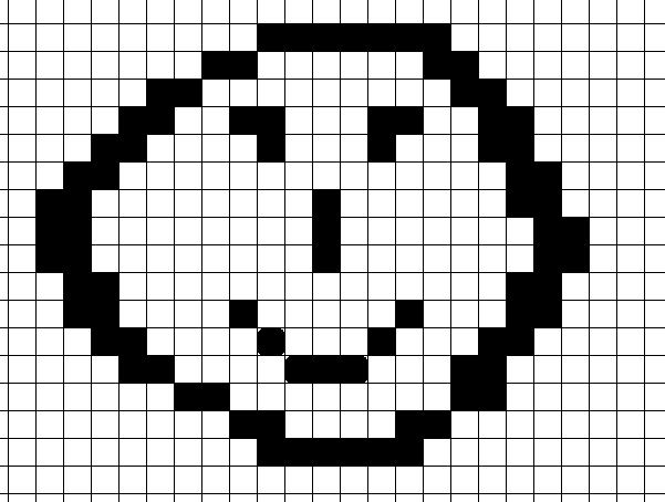
Once again we need to determine what the probability of occurrence for a certain image is in order to classify it.  Therefore, if we can determine the probability of each pixel dependent on the states of the rest of the pixels in the image, we can determine what type of image has the highest probability of being classified.  We know that every classification has certain classes that we want to classify our images into (let's say sad face and happy face).  So what we are looking for is a way to find the which of these two categories has the highest probability based on the individual dependent probabilities.  It turns out that when using Markov Meshes, the conditional probability of a pixel state dependent on a whole array, just simplifies to a pixels' dependence on it's 8 nearest neighbours or:

We can go through the math in a little more detail below:
 
 

The following definitions are needed for the discussion about Markov Meshes.

1)  is an m x n array of discrete random variables that create an array as shown below:

2)  is a variable located in the row a and the column b of .

3)  is the rectangular array of all random variables  with i=<c and j>=d.

4)  is the rectangular array  with the point  deleted.

5)  is a nonrectangular array such that all variables to the left or above  are included.  This is shown in the diagram below.

What we are attempting to do is classify an image based on the assumption that a two dimensional image can be represented as a third order Markov Mesh and the dependencies between pixels can be determined using the dependencies defined by the Markov Mesh.
 

Consider the probability of the state of  conditional on  is equal to the probability of  conditional on the set of the nearest neighbors to  within .

For the third order Markov Mesh we get:

.

If one now considers the joint probability of all variables in the array X_a,b, the Markov Mesh yields the following product:

where p(X_a,b) denotes the joint probability.

We know already from the section on Markov Chains, that a pixel at a location k in a first order Markov Chain depends solely on it's to nearest neighbors:

.

If this extended two a third order Markov Mesh, we obtain the following conditional proabability:

.

As can be seen, the conditional probability of  as it pertains to the entire array,  is the same as the conditional probability of the existence of  as it pertains to its eight nearest neighbors.

The third order Markov Mesh is a special case of this.   The general assumption is that  where U_a,b are the elements of the upper left hand sector of the original pixel array.  From this the probability of existence of a pixel array  can be shown to be:

.
 
 

Previous : 2b.Hilbert Space Filling Curves
Next: 2d. Dependence Trees