2. Context in Image Classification
a. Lower Order Markov ChainsContext in Text Recognition
b. Hilbert Space Filling Curves
c. Markov Meshes
d. Dependence Trees
a. A Quick Bit on Compound Decision Theory
b. Dictionary Look-up Methods
Conclusions
References
2. Context in Image Classification
a. Lower Order Markov Chains Abend
Markov Chains are being covered by another project in this course therefore I will be brief as to the covering the Markov chains in this section, and how they can be useful for image analysis Why would we want to use Markov chains in pattern recognition. Like in the example on the previous page the classification of an image is dependent on all the other pixels in the pixel grid. One would have a very hard time in classifying the following image as an eye if there were to see it all by itself. Clearly in the context of the entire image, it makes sense however.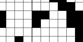
Therefore we need a manner to efficiently look at the dependencies between pixels and how that affects the probability of a certain state to occurring. By state I mean a certain configuration of pixels that form an image. Clearly we want to determine the configuration of pixels which define a class that has the highest probability of occurring
Consider a very simple image, such as a straight line of pixels:

Clearly, this line isn't extremely interesting, nor is it of much use. However it will serve to illustrate the point that needs to be made. In the above image there is a line of pixels which can take on one of two states: black or white (think of this as something like the strip of a bar code). Can we determine some form of dependence between the pixels. For example can we say that since we know the state for all n pixels in our image can we determine the probability of our current pixel being black or white. Or is the decision even that complicated?
Remember that any classification procedure is trying to classify an image into predefined categories. So consider bar code 1 vs. bar code 2 What we need is which of these two bar codes matches what we have above.
It turns out that if we use
a Markov all that needs to be determined is the conditional probability
of the pixels surrounding the current one that we are examining or:![]() .
Also under other conditions we can determine that a Markov Chain is dependent
on the two pixels before and after the pixel we are examining (ie: p(xk|x1x2...xk-1)=p(xk|xk-1xk+1)).
Which makes sense, because essentially we are saying that the state of
your current pixel is only dependent on your two nearest neighbours.
Once we know the probability of occurrence of a certain state, for each
pixel, we can then determine which image has the highest probability of
occurring as a whole.
.
Also under other conditions we can determine that a Markov Chain is dependent
on the two pixels before and after the pixel we are examining (ie: p(xk|x1x2...xk-1)=p(xk|xk-1xk+1)).
Which makes sense, because essentially we are saying that the state of
your current pixel is only dependent on your two nearest neighbours.
Once we know the probability of occurrence of a certain state, for each
pixel, we can then determine which image has the highest probability of
occurring as a whole.
Clearly this concept can be extended to a two dimensional pattern, which will be done when looking at Markov Meshes.
Firstly a few other factors
must be examined prior to examining the use of lower order Markov Chains.
Orthonormal Expansion
Consider a vector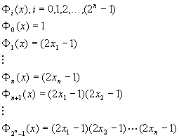
Let p(X) be a probability distribution. If p(X) does not equal zero for all states of the vector X then we can say the following:
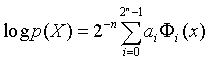
where
![]()
An Approximation Distribution Based on Marginal Probabilities
Let s0 , s1, ..., sk-1 represent the k different subsets of the n variables. The subsets are not necessarily in the same order, however each of the subsets has each value of xi included in at least each of the subsets.Let p(s0 ), p(s1 )...,p( sk-1) represent marginal probability functions for the probability density function of p(x1, x 2,...xn). Then an iterative approach in order to estimate the nth order probability function p(x) is given by the following equation:
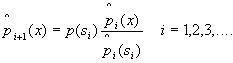
where si
= si (mod k) and ![]() is
is ![]() summed over the variables
not in the subset of k.
summed over the variables
not in the subset of k.
This procedure has the
property that at each stage of the iteration the estimate of ![]() remains a probability distribution and diverges according to
remains a probability distribution and diverges according to ![]() , which is a monotonically decreasing function of i. The divergence
between
, which is a monotonically decreasing function of i. The divergence
between ![]() and it's estimate,
and it's estimate, ![]() continues to decrease until and estimate which is consistent with with
all the given marginal probabilities.
continues to decrease until and estimate which is consistent with with
all the given marginal probabilities.
An Optimal Expansion Recipe for Classification
When a pattern (like an image) can belong to one of two classes with probability distributions p(x) and q(x) respectively, the logarithm of thelikelyhood ratio,
Since there are 2n-1
combinations of the set S possible it is possible to represent the classification
function as the orthonormal expansion given earlier as long as the probability
distributions are specified and non-zero. However computationally
this becomes too large to do as n gets large.
Markov Chains
As was mentioned earlier Markov chains are being covered by a another project in this course. Please take a look.If we examine Markov chains
as a classification method for images, we must first consider an image
pixels as a set of random variables, ![]() ,
where each xi can take on the binary values of 1 or 0.
Markov chains have the property that given the present condition of the
pixel we are examining, the state of the next pixel is conditionally
independent of the pixel that is currently being examined. Or, in
other words:
,
where each xi can take on the binary values of 1 or 0.
Markov chains have the property that given the present condition of the
pixel we are examining, the state of the next pixel is conditionally
independent of the pixel that is currently being examined. Or, in
other words: ![]()
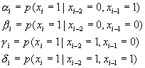
A property of Markov Chains
is that the probability of a link of the chain, or a pixel k (in
this case) as it relates to some other link in the chain, j, is ![]() for all j<k. However for k<n the following property
pertains:
for all j<k. However for k<n the following property
pertains:
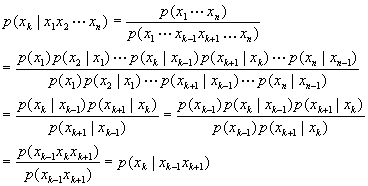
This indicates that any point on the chain (or pixel) has a probability dependent only on it's two nearest neighbours (on either side of the point).
Now consider for a first
order chain:
![]()
In other words consider
the probabilities that the current pixel being examined is a logical 1
i we know the previous pixel. We know that the conditional probability
that the pixel has a value of 0 knowing that the previous pixel is simply
1-![]() or 1-
or 1-![]() .
.
Define xi =0 for all
i<1 and all i>n such that ![]() and
and ![]()
However the state of any point is dependent on only its nearest two neighbors in a one dimensional chain. A set of pixels can be thought of as such a chain where the probability of the state of a pixel being 1 or 0 is dependent on the states of the two pixels around it.
Similarly in the second order
case the probability of the state of the current pixel is dependent on
the state of the four nearest neighbours around the pixel. Of course, this
becomes apparent when we consider the case of a two
dimensional binary image. Let us
know examine the second-order Markov chain and its dependence on it's four
nearest neighbours. Let,
If we expand the joint probability,
we obtain ![]() , ie: the two
neighbors prior to the current pixel, are the only pixels are the only
dependencies for the current pixel.
, ie: the two
neighbors prior to the current pixel, are the only pixels are the only
dependencies for the current pixel.
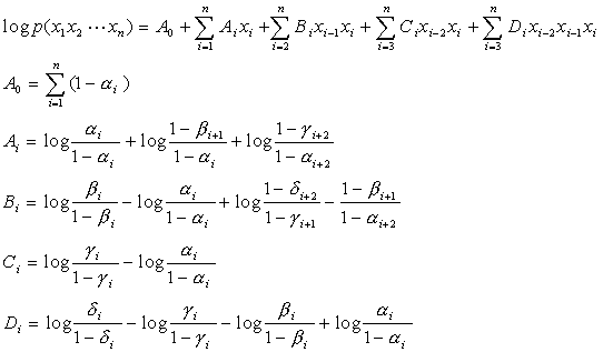
Take the logarithm of both
sides and we obtain:
 .
.
In general this would allow
one to determine is the probability for certain combination of ![]() to occur. if a required estimate for the probability is possible,
then it can be estimated using the orthonormal expansion determined earlier.
If it falls under two different classes then the optimal classifier shown
before can be used in order to determine the class in which the pattern
falls. However in to look at each image pixel by pixel it is important
to determine a manner in which to traverse the pixel grid efficiently.
to occur. if a required estimate for the probability is possible,
then it can be estimated using the orthonormal expansion determined earlier.
If it falls under two different classes then the optimal classifier shown
before can be used in order to determine the class in which the pattern
falls. However in to look at each image pixel by pixel it is important
to determine a manner in which to traverse the pixel grid efficiently.
Previous : 2.
Context in Image Classification
Next:
2b. Hilbert Space Filling Curves